Job Evaluation: Meaning, Methods & Process
What is Job Evaluation?
Job Evaluation is the output provided by Job Analysis. While Job Analysis describes the duties, authority relationships, and skills required for a job, Job Evaluation uses that information to evaluate the worth of each job.
It is a formal and systematic process of comparing jobs to determine the value of one job relative to another. The primary goal is to establish a logical job hierarchy to fix fair wages and salaries.
Key Distinction: It evaluates the JOB, not the PERSON. (Performance Appraisal evaluates the person). It assesses the demands the job makes on a normal worker, ignoring individual abilities.
Key Definitions
-
ILO (International Labour Organization): “An attempt to determine and compare demands which the normal performance of a particular job makes on normal workers without taking into account the individual abilities or performance of the workers concerned.”
-
Kimball and Kimball: “An effort to determine the relative value of every job in a plant to determine what the fair basic wage for such a job should be.”
- “Job evaluation is the process of analyzing and assessing various jobs systematically to ascertain their relative worth in an organization.” — Dale Yoder
Principles of Job Evaluation (The Kress Model)
According to Kress, a successful job evaluation programme must follow these six principles:
-
Rate the Job, Not the Person: The focus must remain strictly on the requirements of the role, not the person currently holding it.
-
Use Definable Elements: The factors used for rating (e.g., skill, effort) should be explainable, limited in number, and cover all job requisites without overlapping.
-
Clear Definitions: The elements selected must be clearly defined and properly selected to avoid ambiguity.
-
Foreman Participation: Supervisors and foremen should participate in rating the jobs within their own departments to ensure accuracy.
-
Employee Cooperation: Employees should be given an opportunity to discuss job ratings; this secures their cooperation and trust.
-
Avoid Too Many Wage Rates: It is unwise to create a unique wage rate for every single point total. Instead, jobs should be grouped into occupational wages.
The 7 Key Objectives
Why do organizations perform Job Evaluation?
-
Standardization: To provide a standard procedure for determining the relative worth of each job.
-
Accurate Descriptions: To secure and maintain complete and impersonal descriptions of every distinct job in the plant.
-
Equal Pay for Equal Work: To ensure that like wages are paid to all qualified employees for similar work.
-
Fair Promotion: To promote fair and accurate consideration of employees for advancement and transfer.
-
Benchmarking: To provide a factual basis for comparing wage rates with similar jobs in the community or industry.
-
HR Decisions: To provide information for selection, placement, training, and work organization.
-
Equitable Pay Structure: To determine a rate of pay that is fair relative to other jobs in the plant.
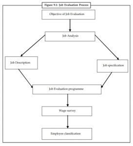
The Job Evaluation Process
The process is a logical flow that transforms job data into a wage structure.
-
Job Analysis: Collecting data via questionnaires, interviews, or observation.
-
Job Description: A written statement of what the job holder does.
-
Job Specification: A statement of the human qualities required to do the job.
-
Job Evaluation Programme: Choosing the method (Ranking, Point, etc.) to assess the jobs.
-
Employee Classification: Grouping similar jobs into grades or categories.
-
Wage Survey: Checking market rates for “Key Jobs” to ensure external competitiveness.
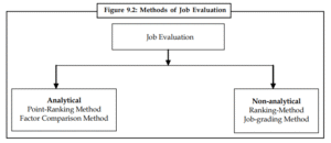
Methods of Job Evaluation
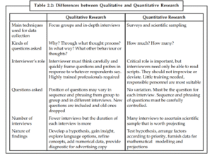
Methods are broadly classified into Non-Analytical (Qualitative) and Analytical (Quantitative).
A. Non-Analytical Methods (Qualitative)
These methods treat the job as a whole and do not break it down into detailed factors.
1. Ranking Method
This is the simplest form. The committee assesses the worth of each job based on its title or content and arranges them in order of importance.
-
Example: CEO > Manager > Clerk > Peon.
-
Pros: Easy and cheap for small companies.
-
Cons: Very subjective; doesn’t say how much more valuable one job is than another.
The 5-Step Mechanism:
-
Preparation of Job Description: Essential to resolve disagreements among raters.
-
Selection of Raters: Usually a committee. Jobs are often ranked by department (clusters) to avoid comparing dissimilar jobs (e.g., factory vs. clerical).
-
Selection of Key Jobs (Benchmark Jobs): 10 to 20 representative jobs are selected first to establish a rough rating scale.
-
Ranking of All Jobs: All other jobs are compared to the Key Jobs and ranked from “lowest to highest.”
-
Job Classification: The ranked list is divided into groups (usually 8 to 12), and wage ranges are assigned to each group.
Factors used for Ranking:
-
Supervision of subordinates.
-
Cooperation with associates.
-
Probability/Consequences of errors.
-
Minimum experience requirement.
-
Minimum education required.
Pros & Cons:
-
Merit: Simple, inexpensive, less time-consuming.
-
Demerit: Subjective (based on personal bias), does not tell how much more valuable one job is than another.
2. Job Classification (Grading) Method
In this method, the number of grades is decided first, and then jobs are fitted into these grades. This is common in Government jobs.
The 5-Step Mechanism:
-
Job Description: Gather basic job info.
-
Grade Description: Define specific levels or grades (e.g., Grade 1 = Routine work, Grade 2 = Skilled work). Each grade must be distinct.
-
Selection of Key Jobs: Select 10-20 jobs covering all departments.
-
Grading Key Jobs: Assign key jobs to appropriate grade levels.
-
Classification: All remaining jobs are matched against the grade definitions and classified.
Pros & Cons:
-
Merit: Administratively easy for pay determination. Widely used in government services.
-
Demerit: Rigid system. It is difficult to write grade descriptions that fit a large, diverse organization.
B. Analytical Methods (Quantitative)
These methods break jobs down into components (factors) and assign scores.
3. Point Ranking Method
This is the most widely used and systematic method.
The 5-Step Mechanism:
-
Select Job Factors: Choose compensable factors like Skill, Responsibility, Effort, and Working Conditions.
-
Construct a Scale: Assign point values to each factor (e.g., Skill = 50% weight). Divide factors into degrees (Degree 1, Degree 2) and assign points to degrees.
-
Evaluate Jobs: Analyze every job and award points for each factor based on the scale.
-
Design Wage Structure: Sum the points to find the total job worth.
-
Adjust Wages: Convert points into monetary values.
Pros & Cons:
-
Merit: The worth is determined by distinct factors, not just “overall feel.” It is systematic and easy to explain to employees.
-
Demerit: Developing the point scale is complex and time-consuming.
4. Factor Comparison Method
This method ranks jobs by comparing them factor-by-factor against “Key Jobs.”
The 5 Universal Factors Used:
-
Mental Requirements
-
Skill Requirements
-
Physical Exertion
-
Responsibility
-
Job Conditions
Mechanism: Instead of points, this method often assigns a monetary value to each factor. Each job is ranked against others for each of the five factors individually.
Pros & Cons:
-
Merit: Can evaluate unlike jobs (manual vs. clerical) using the same set of factors.
-
Demerit: Highly complicated and expensive to install.
Critical Appraisal: Advantages vs. Limitations
Advantages (Why use it?)
-
Removes Inequality: Helps maintain consistent wage differentials.
-
Reduces Grievances: Provides an objective basis for wages, improving labor relations.
-
Standardization: Replaces accidental wage bargaining with impersonal standards.
-
Better Recruitment: Information from analysis improves selection, transfer, and promotion.
-
Simplifies Administration: Leads to greater uniformity in wage rates.
Limitations (The Drawbacks)
-
Rapid Changes: Technology changes job contents quickly, making evaluations outdated.
-
Market Mismatch: Internal evaluation may not match external market rates (supply and demand).
-
Cost & Time: It takes a long time to install and requires specialized technical personnel.
-
Employee Anxiety: It creates fear and doubt in the minds of employees when first introduced.
-
Rigidity: Implementing substantial wage changes may be restricted by the firm’s financial limits.
If you have doubt in above topic you can prefer watching this video. (LINK)